Modeling Basin Infilling Processes in Estuaries using two different approaches: An Aggregate Diffusive Type Model and a Processed Based Model*

Modelação do Preenchimento Sedimentar em Estuários. Comparação de duas abordagens: Modelo Difusivo de Parâmetros Agregados e Modelo de Processos Físicos

 

P. Laginha Silva^@,I, F. Martins^I, T. Boski^I, R. Sampath^I

^@Corresponding author: pisilva@ualg.pt
^IUniversidade do Algarve – CIMA, Campus da Penha 8005-139 Faro, Portugal. E-mails: pisilva@ualg.pt, fmartins@ualg.pt, tboski@ualg.pt, rmudiyanselage@ualg.pt

 

ABSTRACT

Long term basin infilling simulations are traditionally carried out using synthetic models. The usual reasons for the preference of these types of models over the more elaborated process based models are the heavy computational needs and the poor knowledge of the processes in presence.
The main objective of this article is to show that computational power and numerical methods are now reaching a state that these long term simulations can be affordably obtained using state-of-the-art process-based models. To accomplish this, the morphodynamic model, that solves explicitly the mass conservation equation for the bathymetry evolution and then actualizes the bathymetry, are used to perform long term simulations for the estuarine bathymetry evolution.
The results are compared with a traditional synthetic aggregate parameters basin infilling model of the diffusive type. It is shown that the process based models, while conceptually different, produce physically meaningful and comparable results with the diffusive type models. Moreover, they enable the simulation of conditions not allowed by the formulation of diffusive type models with acceptable computational times, as for example the addition of tide and river input.

Palavras-chave: Morphodynamic modeling, Basin infilling, sediment dynamics, aggregate diffusive type model, Process Based Model.

---

RESUMO

As simulações de preenchimento sedimentar de longo termo são tradicionalmente realizadas através de modelos de parâmetros agregados. A justificação invocada para a utilização desses modelos em vez dos modelos baseados em processos físicos, mais elaborados, relaciona-se com as maiores necessidades computacionais destes últimos e com fraco conhecimento dos processos presentes.
O principal objectivo deste artigo é mostrar que actualmente o poder computacional e os métodos numéricos possibilitam que essas simulações de longo-termo possam ser resolvidas utilizando modelos de processos físicos. O modelo Mohid para além de ser morfodinâmico resolve ainda a equação de conservação de massa para a evolução da batimetria que depois actualiza a batimetria.
Os resultados são comparados com os obtidos por um modelo difusivo de preenchimento sedimentar tradicional. Embora conceptualmente diferentes, os modelos baseados em processos produzem resultados fisicamente significativos e comparáveis com os modelos do tipo difusivo. Os modelos baseados em processos permitem a simulação de condições impossíveis de formular com os modelos do tipo difusivos em escalas temporais computacionalmente aceitáveis.

Keywords: Modelação Morfodinâmica, Preenchimento Sedimentar, Dinâmica Sedimentar, Modelo Difusivo de Parâmetros Agregados e Modelo de Processos Físicos

 

1. Introdution

Estuarine sediment transport presents a great challenge for scientists and coastal engineers. The interaction between the fluid (water) and the solid (dispersed sediment particles) phases is crucial in morphodynamics. The process of sediment transport and the resulting morphological evolution of estuaries gets more complex with the exposure of the estuarine systems to the natural and variable environment (climatic, geological, ecological, social, etc.).

The last half century has seen more and more developments and applications of mathematical models for estuarine flow, sediment transport and morphological evolution. The first attempts for a quantitative description and simulation of basin filling in geological times started in the late 60´s of the last century (eg. Schwarzacher, 1966; Briggs & Pollack, 1967). An excellent synthesis of basin quantitative models can be found in Allen and Allen (1990). However, the quality of this modeling practice has emerged as a crucial issue of concern, which is widely viewed as the key that could unlock the full potential of computational estuarine hydraulics. Cao & Carling (2002) identify that the major factors affecting the modeling quality comprise of: (a) poor assumptions in model formulations; (b) simplified numerical solution procedure; (c) the implementation of sediment relationships of questionable validity; and (d) the problematic use of model calibration and verification as assertions of model veracity.

Most of the models used to study fluvial basin filling are of the “diffusion type” (Flemmings and Jordan, 1989). It must be noted that these types of models do not assume that the sediment transport is performed by a physical diffusive process. Rather they are diffusive type models based on mass conservation. In the “synthesist” viewpoint (Tipper, 1992; Goldenfeld & Kadanoff, 1999; Werner, 1999) the dynamics of complex systems may occur on many levels (time or space scales) and the dynamics of higher levels may be more or less independent of that at lower levels. In these types of models the low frequency dynamics are controlled by only a few important processes and the high frequency processes are not included. Contrary to this is the “reductionist” viewpoint that states that there is no objective reason to discard high frequency processes. In this viewpoint the system is broken down into its fundamental components and processes and the model is built up by selecting the important processes regardless of its time and space scale. This viewpoint was only possible to pursue in recent years due to improvement in system knowledge and computer power (Paola, 2000).

Even thought the assumptions are different, Gabriel & Martins (2008) had demonstrated the applicability of a process based model (MOHID model (Miranda et al., 2000)) in morphodynamic simulations to study the evolution of the estuarine bathymetry in a time scale of thousands of years through a comparison with similar simulations of both an idealized synthetic model and an intermediate model. They had compared the bed evolution during the first 750 years with the equilibrium profile obtained by Schuttelaars and Swart (2000) and with an intermediate, process-based, linearized model (Hibma et al., 2003) for the same geometry and conditions of simulation. In that work the evolution of a 1D estuary bed profile during 10000 years by MOHID model shows similar trends for most of the basin and a clear equilibrium tendency, achieved after the first 2000 years of simulations.

The primary aim of this paper is to demonstrate that it is possible to simulate the evolution of the estuarine bathymetry through a process-based hydrodynamic, sediment transport and morphodynamic model, solving explicitly the mass and momentum conservation equations. With this objective, a comparison between two mathematical models for alluvial rivers is made to simulate the evolution of the estuarine bathymetry of a conceptual 1D embayment for periods in the order of a thousand years. Although the selected bathymetry grid is a conceptual estuary its generic configuration is the same observed in the Guadiana estuary and the water and sediment discharge are typical of this estuary.

The traditional diffusive type model based on the diffusion equation (Paola, 2000), used in the “synthesist” viewpoint and the process-based model MOHID (Miranda et al., 2000) are used. The results are also used to highlight some of the uncertainties inherent in such models.

A process based model is a dynamic model that is based in mathematical formulations of the more relevant physical processes. The process based model is explored to investigate the combined effect of tide, sea level rise and river discharges in the behavior and sensitivity of the estuary system. These effects cannot be simulated using the diffusive type model, due to its intrinsic assumptions.

The next sections present a brief description of the synthetic diffusion model and the limited capabilities of these types of models are highlighted. Then the major features of the process based model are described. Subsequently, the simulations layout is introduced; the results are presented and discussed. Finally the principal conclusions of the work are listed.

 

2. Model description

2.1 The diffusion model and its dependencies

The basic flow equation, the continuity and Navier-Stokes equations describing (fluid) mass and momentum conservation may be considered exact at least for a pure fluid. In contrast, much remains unclear as far as the basic governing equations for sediment are concerned. Unlike “molecular” scalars like salinity or temperature, sediment constitutes a separate physical phase, the motion of which may not necessarily be the same as the motion of the fluid. The large bulk of the work on sediment transport modeling has been based on a continuum approach, where only a sediment mass conservation equation is taken, without mention of sediment momentum conservation equation (Lyn, 2007).

Described by Chris Paola (2000), the diffusion model is based on the standard diffusion equation:

 

 

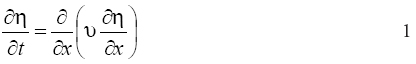
Where ? is the elevation of bed level (m), t time (s), x downstream distance (m) and ? the transport (diffusion) coefficient.

Diffusion is a physical process that occurs in a flow in which some property is transported by the random motion of the molecules. Diffusion is related to the stress tensor and to the viscosity. Turbulence and the generation of boundary layers are the result of diffusion in the flow. The mixing process responsible for the distribution of quantities of heat, dissolved gas and solids, and suspended sediment, is shown to consist of a uni-directional movement by turbulent mean flows, called advection, and a three-dimensional spreading action produced by the turbulent flow components, called diffusion.

The type of model described in this chapter does not assume that the sediment transport is performed by the physical diffusive process referred in the previous paragraph since it is a synthetic model based on the conservation of mass:

 

 

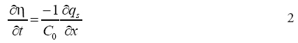
Where q_s is the mean sediment flux per unit width of basin (m²/s) and the volume sediment concentration in the deposits. The diffusive nature of the Equation 2 arises from the assumption of a slope-dependent sediment flux:

 

 

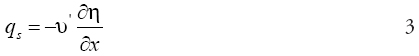
Where ? = ? C₀ . The physical meaning however is of a mass conservation equation; the diffusion coefficient embodies the parameterization of the sediment flux q_s. The diffusion equation is a mass conservation equation where the flux is parameterized as a function of the bottom slope. Instead of invoking diffusion as a mean behavior (i.e. Eq. 1), the model behaves diffusionally in aggregate.

One problematic assumption for geophysical simulations is that the dimensionless (or Shields) stress t* must be constant within particular fluvial regimes in time and space, a difficult assumption to make in real scenarios. This is a substantial generalization, of the approach presented in Paola et al. (1992). With t* defined as:

 

 

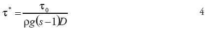
Where t₀ is the bottom shear stress (Pa), ? is the fluid density (Kg/m3), s the sediment specific gravity and D the median grain size (m). This is obviously difficult to accomplish in real life situations. The bottom shear stress is used for the determination of the diffusion coefficient, as part of the formulation of the diffusion model. In this work the diffusion coefficient parameter wasn't determined by the model, instead it was considered constant and adjusted to minimize the longitudinally integrated error between the diffusive model and the MOHID model.

Another very stringent assumption for the applicability of the diffusion model in real life situations is that boundary conditions, such as sediment supply and river flow, must be constant. The formulation of diffusive models makes impossible the inclusion of these processes. The simulation of time dependent processes, such as the impact of climate change, is thus difficult to accomplish with such models.

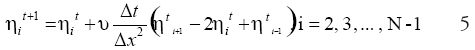
The model was implemented in FORTRAN 95 language using the finite differences method and an explicit temporal discretization of Equation 1:

 

 

 

2.2 The process based model and its implementation

The implementation of the process-based morphodynamic simulation is based on the finite volume MOHID modeling system. It is an open access code developed over the last 30 years in the IST (Technical University of Lisbon, Portugal). It has originally been developed for short time simulations (days to years) and is now being applied for the first time in geologic timescale studies. It is a modular system that includes, among others, models for hydrodynamics, sediment transport and sediment bed evolution (Bernardes et al., 2006).

The system architecture is object oriented (Miranda et al., 2000). The velocity fields are computed in the hydrodynamic module, using a 3D formulation with hydrostatic and Boussinesq approximations (Martins et al., 1998).

The equations are solved using the finite volume method with an ADI (Alternate Direction Implicit) discretization. The resulting equations are obtained by integration of the Navier-Stokes equations over the cells:

 

 

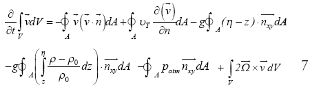
Where v is the velocity vector, V the cell volume, n the normal to the cell and O the velocity of the Earth rotation. Although Equation (7) is the more general 3-D equation which is part of MOHID, in the present application the 1D-vertically integrated version of this equation is used.

In the vertical direction a generic discretization method is implemented (Martins et al., 2001). At the open boundaries both imposed values and radiative conditions can be set (Coelho et al., 2002). In tidal flats, a moving boundary condition is implemented enabling the drying and flooding of cells as a function of the water level. The bottom stress is implemented implicitly using a quadratic law.

The bed evolution is computed solving the mass balance equation:

 

 

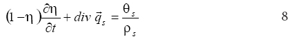
Where n is the sediment porosity, Ts is the sediment flux between the water column and the bed (Kg/(m²/s) and ?s is the dry sediment density (kg/m^s). In this equation: q_s is the total sediment flux per unit width consisting of bed load and suspended load.

The bed load fluxes are computed in an orthogonal grid system of the Arakawa C type (Arakawa and Lamb, 1977). In each centre cell (Z point) the transport flow is computed. In order to compute the sediment transport in an estuary the formulation of Ackers and White (1973) is chosen. These authors developed a total transport formula for fine and coarse sediments exposed to unidirectional water current. The expression assumes that the coarse sediments are transported near the bottom, at a proportional rate to the shear stress, while the fine sediments are in a suspended load due to turbulence. The turbulence intensity depends of the energy dissipation generated by the bottom friction, resulting in a suspended load depended of the bottom shear stress. Although we had used a 1-D vertically integrated model, the MOHID model still uses the integral formulation of Ackers-White. In this 1D case, the MOHID model calculates the fluxes using the Ackers-White formulation that parameterizes the different types of sediment transport.

In a second step the different flow constituents are interpolated: the Zonal (or X) component is interpolated to the U points and in the case of 2D grid the Meridional (or Y) component is interpolated to the V points. In case of a 3D grid, to estimate the evolution of the sand thickness in the cell center (Z point) a mass balance is done.

The availability of sand in a cell is limited by the depth of the bed rock.

The system combines a model of hydrodynamic circulation (the MOHID model) with a model of transport for non-coesive sediments (module SAND). This system computes the turbulence averaged currents and determines the bathymetry evolution and its feedback action in the circulation (Martins et al., 2001).

 

3. Simulation layout

The diffusive type model had a simulation layout similar to the MOHID model, trying to approximate both models to the same initial parameters, as for example: boundary conditions, grid formulations, discharge values and others.

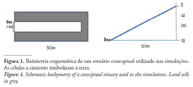
A schematic bathymetry of a tidal basin was constructed with 50 cells of 1 Km by 1 Km size, covering an area with 50 km length and 1 km width (Figure 1). The initial bed depth was imposed with a linear variation from 0 m at the head of the estuary to 10 m at the mouth. By convention the depth values are assumed to be positive, negative values denoting positions above the sea level.

A continuous run of 1000 years was performed with the MOHID model and the diffusive type model. For the MOHID model simulations a typical total river flow of 332,15m³/s with a sediment concentration of 1kg/m³ was divided among five upstream cells of the estuary and every concentration discharge was injected in each cell starting 48 km until 44 km dowstream, identical to the simulation layout of the diffusive type model. The river discharge values were selected as the mean flow and the highest sediment concentration observed on the Guadiana basin, on the hydrometric and sedimentologic station Pulo do Lobo (SNIRH, 2009).

From the same INAG database (SNIRH, 2009) it was used the annual flow distribution although it doesn't have a full 100 years extent time series of the daily mean flow because the registries only started after October 1940. As a result, the temporal flow distribution used in this simulation consists of a 100 year replication by a one year record in the station Pulo do Lobo (reference 27L/01H). The year 1960 was selected as a representative flow distribution in this area due to be a heterogeneous year with two main annual events of higher flows.

The SNIRH database does not possess for Pulo do Lobo station a correspondent sediment distribution, but only a group of scattered measurements of sediment concentrations during a four year period from February 1982 to February 1985. To construct a temporal series of sediment concentration the higher sediment concentration was chosen as representative of a worst case scenario and a direct distribution relationship between sediment concentration and flow was performed.

For stability reasons the time step (?t) used in the MOHID model was set to 60s (Courant number = 1.3835).

For all the MOHID model simulations, a null gradient boundary was applied at the open ocean boundary. This type of boundary assumes that the sediment concentration at the open boundary during ebb is equal to the interior concentration adjacent to the boundary. During flood, the concentration of sediment entering the system is obtained from a first order relaxation equation to a fixed exterior value with an infinitely large decay time. The standard method follows the equation:

 

 

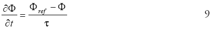
Where F is the relaxed variable, corresponding to the concentration at the open boundary, F_ref is the reference external value and t is the relaxation time scale. The variable t controls the mixture between the property offshore and the property inside the estuary that runs out during ebb time. If t is too large the boundary value is equal to F_ref (instantaneous mixture).

The MOHID model does not have a fix bottom elevation on the open boundary as the diffusive type model, enabling the formulation of a tidal wave entering the estuary.

The system was also forced by tide in the open boundary by its most important component: a single M₂ tide with constant amplitude of 1.75 m and a reference vertical level (hydrographic zero). The value used is normally used as the reference level in Portugal due to the lowest low tide in the coastal and estuarine zones in Portugal, which in the Port of Lisbon was register as equal to 2.2m.

To validate the results, several MOHID simulations were performed with non-cohesive sediment typical of medium sand with a d₅₀ value of 400 µm (Wentworth, 1922) being this the representative value for the sediment existing in the Guadiana Estuary Basin.

Just as an example, with the characteristics referred previously, the MOHID model takes approximately 7h to obtained results for a 100 years run with a 2.3GHz dual-core Intel Core i5 processor.

In the case of the diffusive type model, the grid is the same used by the MOHID model with identical number of mesh points, 50 cells (N). A constant time step ?t (86400s) was used. t_max is the duration of the simulation (seconds). In this case 1000 years was considered.

As already mentioned in the chapter 2 – Model Description, the diffusion coefficient of the model was adjusted to minimize the longitudinally integrated error between the diffusive model and the MOHID model. The value of the diffusion coefficient (?) was considered constant in all the system and equal to 0.077m²/s.

In the grid cells with discharge points (described below), a sediment source, S_sed, was added to Equation 5:

 

 

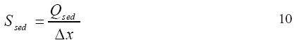
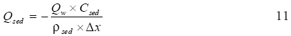
Assuming that Q_sed is the sediment flux (m²/s) obtained by Equation 8 and equal to -2.5 x 10^-5 m²/s, where Q_w is the water discharge (m³/s), C_sed the sediment concentration (kg/m³) and ?_sed the sediment density (kg/m³). Note that Q_sed is a negative value due to the localization of the source be on the right of the grid.

 

 

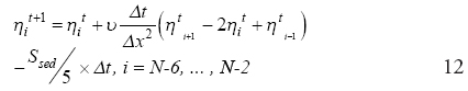
The S_sed was divided in five discharge points among the five upstream cells of the estuary, from a downstream distance of 44 km to 48 km. For this grid cells Equation 5 becomes:

 

 

In this type of model it is not possible to add to the simulations any other estuary processes like the water river discharge, the tide or the sea level rise. Instead the water motion is driven by point sources from a downstream distance of 44 km to 48 km.

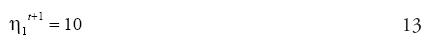
In the boundary limits, cells 1 and N, different assumptions were implemented: In the open boundary, cell 1, ? was assumed to be constant in time and equal to 10m:

 

 

Near the river boundary, last grid cell, it was imposed a gradient boundary condition, where the variable ? was assumed to be the same of grid cell N-1 in time t+1:

 

 

4. Results

Both models have different physical assumptions and for this reason the results obtained with the two models will not be equivalent. Nevertheless, the main assumptions are the same: 1D schematic bathymetry, bathymetry gradient along the estuary and sediment discharge. In the subsequent sections the results obtained with each model are presented.

4.1 Results of the diffusive type model

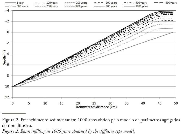
With the diffusive type model it was possible to simulate 1000 years evolution of the sediment bathymetry showing a progressive infilling of the estuary basin (Figure 2).

In the analysis of the results it must be noted that the basin infilling process obtained by this model is the result of the simplified process acting as a diffusive wave. It can be observed that the sediment piles up along the estuary with time in a quasi-equilibrium fashion. This result reveals typical behavior of diffusion, showing a constant gradient of the bottom elevation. The diffusion model results only have in stationary regime a constant gradient. At the end of 1000 years this final solution tends to a linear solution. The intermediary solutions (transients) could not be linear but due to the fact of the evolution is too small these transient solutions are approximately linear.

With the analysis of the results from the diffusive type model, it is not possible to observe any erosive process or other physical process that acts in a real estuary basin except the consequent elevation of the sediment bathymetry. At the open boundary, the bottom elevation is fixed in the formulation of the diffusion model, not allowing any erosion or deposition of sediment to be observed in this point.

The results accomplished by the diffusive model confirm the major drawback of these models: to achieve erosion a negative diffusion coefficient would be needed. Quantitatively the results show a maximum sediment deposition upstream with 4m of sediment accumulation decreasing downstream without any sediment deposition observed at the estuary.

4.2 Results of the process based MOHID Model

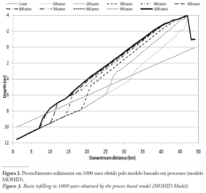
The results obtained by the MOHID model, for the same 1000 year simulation are presented in Figure 3. As already referred in the Simulation Layout chapter, by convention the MOHID model in its formulation assumes depth values positive and positions above the sea level negative.

The bed evolution shows a less diffusive character when compared to the diffusive model. This is expected since the process based model explicitly includes the physical processes controlling the sediment transport and consequently the bed evolution. In fact, the bottom develops as a result of a river discharge with water and sediment input. Also, by physical processes that drive the hydrodynamic and the sediment transport. All this physical processes described before and included in the formulation of the model MOHID permits results physically more credible than the diffusive solution.

The quasi-equilibrium nature of the results are thus not observed, being alternatively observed a transient evolution of the infilling wave.

As the simulation advances in time, the results of the MOHID model show a tendency for a stationary state similar to the one attained with the 1000 year simulation from the diffusive type model. The main difference observed in the process-based model results is that the erosion process is visible in the lower part of the estuary basin, due to the tidal energy, a process not included in the diffusive model. The erosive process reaches a maximum value of approximately 2 meters at the mouth, and is present up to 32 km from the mouth before the infilling wave reaches that position. It can also be observed that both models attain a maximum sediment height of 4 meters near the head. It should be noted that in the process based model the last two cells remain constant because they are used as a boundary condition.

4.3 Behavior and sensitivity of the process based model

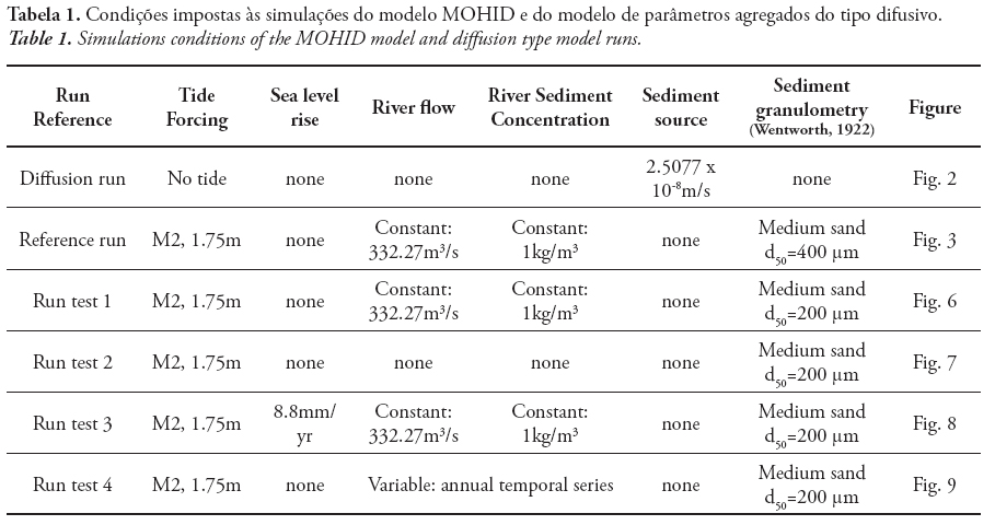
The previous set of simulations has helped to compare both models and to understand its behavior. A subsequent set of 100 year simulations were prepared to show the practical applicability of the process based model and to study the sensitivity of the system to variations in sediment characteristics and forcing. The diffusive model cannot be applied to these situations due to its formulation. Table 1 summarizes the conditions of each simulation, including the reference simulations described in sections 4.1 and 4.2.

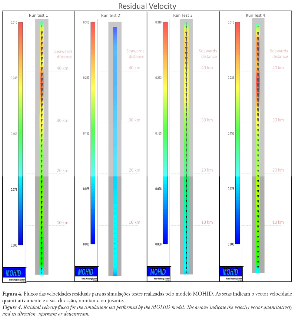
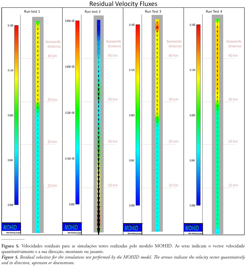
The Figures 4 and 5 summarizes the results of the MOHID model for the Residual Velocity (Figure 4) and Residual Velocity Fluxes (Figure 5).

The Residual Velocity is a time averaged velocity (m/s) during the period of the simulation and the Residual Velocity Fluxes is a time averaged specific flow divided by the average grid cell thickness in m/s which is the specific flow (m²/s) divided by the average thickness of the grid cell in meters during the period of the simulation.

The purpose of the Run test 1 is to understand the influence of the sediment properties on the infilling process. The reference run (Figure 3) uses medium sand with a granulometry of 400 µm. These results are compared to the results of Figure 6 obtained using fine sand with a granulometry of 200 µm.

It can be seen that the infilling process does not evolve in this system when a fine sand supply is used. Moreover, if the initial bed sediment is of the same type, as is the case in this simulation, the system starts to erode until an equilibrium state is reached. This is a physically plausible evolution that could not be achieved by the traditional diffusive models where erosion cannot be accounted for. The bottom evolution observed in the Run-test 1 (Figure 6) could be corroborate with the residual velocities of the system (Figure 4). At the river point of discharge is detected a light increase of the velocity (Figure 4), causing an erosive process that transports sediment and deposits immediately afterwards at 43km seawards (Figure 5). Due to this fact, the water column depth diminishes leading the velocity to increase (Figure 4) and consequently the existence of a new erosive event (Figure 6). Afterwards the velocity stabilizes but still capable of eroding the sediment bottom.

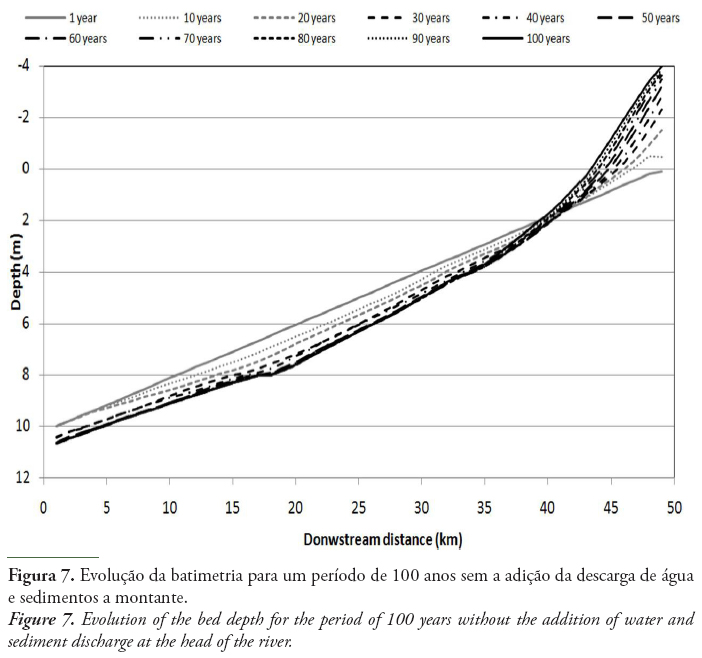
The purpose of the second test is to understand how river forcing modifies the morphodynamic evolution. To evaluate this, the Run-test 2 (Figure 7) was performed without the forcing of river discharge (water or sediment) only with tide.

The results of the Run-test 1 (Figure 6) present the expected erosion at the head of the estuary when compared with the Run-test 2 (Figure 7). The run of Figure 7, without river discharge, displays a pronounced sediment accretion on the head of the estuary. This is due to the lack of energy in that region to promote erosion. In reality the tidal wave is deformed resulting in a tidal asymmetry that favors downward sediment transport in the lower reaches and landward transport in the upper reaches, resulting in the accumulation visible in Figure 7.

This phenomenon is possible to observe in Figure 5 where the first two cells RunTest2 are visible a reversal of the direction of the residual velocities fluxes, with the first two cells having an upstream direction. In the rest of the system, the residual velocity fluxes (Figure 5) are directed downstream, justifying the loss of sediment downstream through the increase of the residual velocities fluxes. The residual velocities (Figure 4) only show very small velocities in all the system in general, with higher residual velocities downstream.

Between 40 and 30km upstream the residual velocities fluxes (Figure 5) inverts and increases and the residual velocities show a considerable higher values. These phenomena could be explained by velocities reaching the capability of remobilize sediment. For this reason it's possible to observe the sediment accumulation upstream (Figure 7) being maximum only in the first cells and decreasing downstream until no more sediment accumulates and the velocities fluxes shows the capability of remobilize the sediment in the system and thus eroding the river bottom.

Still, between 30 and 25km seawards the residual velocity fluxes decreases. This event corresponds to the same area that is displayed in Figure 7 where is visible a reduced erosion. From 25km downstream, the residual velocity and velocity fluxes increase being higher in the last cell, corresponding to the erosive process observed in the Figure 7 in this same area.

Note that the results achieved for this run-test 2 corresponds to residual velocities fluxes very small when compared with the other runs. A possible explanation could be related to the only system forcing be a tidal wave entering the estuary through the open boundary, in opposition with the other run-tests that all have a water and sediment discharge at the head of the river.

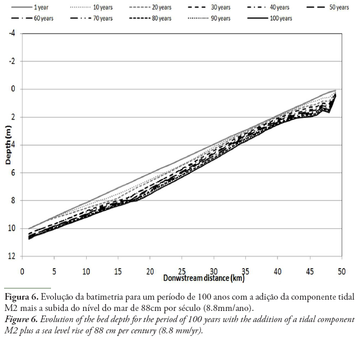
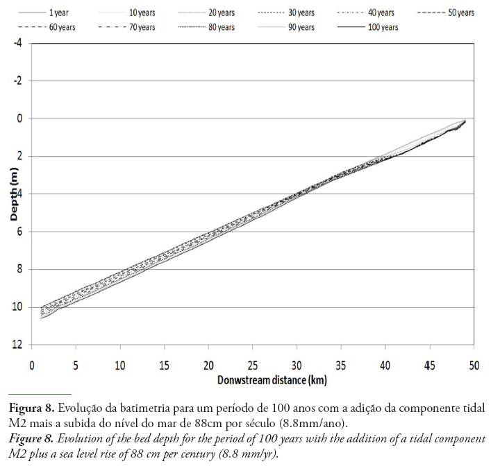
The effect of sea level rise was then investigated in the third test, adding to the M2 tidal wave of the ocean boundary a value of 88 cm per century with the objective of simulate the global sea level rise (SRES, 2001). This value was chosen as the model maximum of the total sea level change for the worst scenario given by the Special Report on Emissions Scenarios (SRES). The SRES was prepared in 2001 by the Intergovernmental Panel on Climate Change (IPCC) for the Third Assessment Report (TAR). The river discharge of water and sediment was maintained constant. The results obtained in this simulation can be observed on Figure 8.

The results obtained show that sea level rises produces globally, much smaller erosion (Figure 8) when compared with the constant level situation (Figure 6) present in the Run-test 1. A slight sediment accretion zone can also be identified in the middle part of the estuary. This behavior is confirmed by classic infilling models that show a strong correlation between basin infilling and sea level rise (Paola et al., 2000). The residual velocities and velocities fluxes (Figure 4 e 5) shows a higher residual velocity at 45km upstream that get smaller from this point seawards. These results demonstrate smaller residual velocities and velocities fluxes when compared with the Run-test 1, confirming the assumption documented previously.

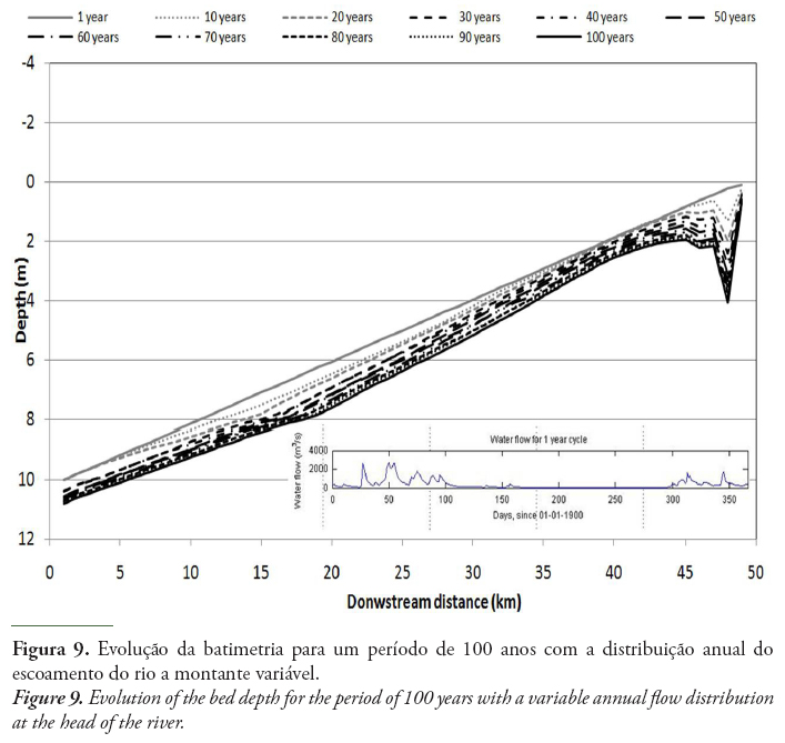
Finally to examine the influence of constant versus variable river discharge, a fourth test was implemented, including a variable annual flow distribution at the head of the estuary and a tidal forcing without the addition of the sea level rise. The results for this simulation can be observed in Figure 9 and shall be compared with the Reference run (Figure 3).

The results show a remarkable erosion process on the head of the estuary, resulting from the increase in river velocity (Figure 4) caused by the river discharge and consequent erosion capacity. Immediately, seaward of this area the estuary bed stabilizes, with the sediment supply and the erosion process acting in an almost equilibrium way. Further downstream of the estuary, higher erosion processes occur along the estuary bed similar to the results already achieved in Run-test 2 (Figure 4, 5 and 8), with the difference that the residual velocity fluxes are higher than in the Run-test 2 due to the sediment availability from the erosive process close to the river discharge.

 

5. Final conclusions

The results presented show that the current computational power and numerical modeling techniques enable the use of process based models, which explicitly describes the physical processes, to simulate long term basin infilling processes. The simulation of the estuarine bathymetry evolution achieved by the process-based model MOHID present the same trend obtained using the traditional diffusion model. Additionally, more detailed simulations are possible due to the physical processes included in the process-based model. In the MOHID results it is possible to observe more comprehensive and realistic results because this type of model includes processes that are impossible for a diffusive type model to describe. Due to this, it was possible to investigate the combined effect of tide, sea level rise and river discharges in the process based model. The results demonstrate the feasibility of using process based models to perform studies with a time scale of 10000 years. This is an advance relative to the use of diffusive type models, enabling the use of variable forcing.

In the future the process based model will be confronted with geological data of the Guadiana estuary to evaluate the similitude of the results.

 

Acknowledgements

This work was supported by the EVEDUS PTDC/CLI/68488/2006 Research Project.

 

References

Ackers, P.; White, W.R. (1973) – Sediment Transport: New Approach and Analysis. Journal of the Hydraulics Division (ISSN: 0044-796X), 99(11):2041-2060. ASCE - (American Society of Civil Engineers), Reston, Virginia, U.S.A.         [ Links ]

Allen, P.A.; Allen, J.R. (1990) – Basin Analysis: Principles and Applications. 445p., Blackwell Scientific Publications, Oxford, U.K. ISBN: 0632024232        [ Links ]

Arakawa, A.; Lamb, V.R. (1977) – Computational design of the basic dynamical processes of the UCLA general circulation model. In: J. Chang (ed.), Methods in Computational Physics, 17: 173-265, Academic Press, New York, NY, U.S.A. ISBN: 0124608175.         [ Links ]

Bernardes, M.E.C.; Davidson, M.A.; Dyer, K.R.; George, K.J. (2006) – Towards medium term (order of months) morphodynamic modelling of the Teign estuary, UK. Ocean Dynamics, 56(3-4):186-197. DOI: 10.1007/s10236-005-0039-9.         [ Links ]

Briggs, L.I.; Pollack, H.N. (1967) – Digital model of evaporate sedimentation. Science, 155(3761):453-456. DOI: 10.1126/science.155.3761.453.         [ Links ]

Cao, Z.; Carling, P.A. (2002) - Mathematical modeling of alluvial rivers: reality and myth. Part 2: Special issues. Proceedings of the Institution of Civil Engineers Water & Maritime Engineering, 154(4):297-307. DOI: 10.1680/wame.2002.154.4.297.         [ Links ]

Carter, T.R.; la Rovere, E.L. (2001) - Developing and Applying Scenarios. In: McCarthy, J.J.; Canziani, O. F.; Leary, N.A.; Dokken, D.J.; White, K.S. (eds.), Climate change 2001: impacts, adaptation and vulnerability, pp.145-190, Third Assessment Report of the Intergovernmental Panel on Climate Change (IPCC), Contribution of Working Group II, Cambridge University Press, Cambridge, U.K. ISBN: 0521807689. Available: http://www.grida.no/climate/ipcc_tar/wg2/pdf/wg2TARchap3.pdf

Coelho, H.; Neves, R.; White, M.; Leitão P.; Santos, A. (2002) - A Model for Ocean Circulation on the Iberian Coast. Journal of Marine Systems, 32(1-3):153-179. DOI: 10.1016/S0924-7963(02)00032-5.         [ Links ]

Flemmings, P.B.; Jordan, T.E. (1989) – A synthetic stratigraphic model of foreland basin development. Journal of Geophysical Research (ISSN 0148–0227), 94(B4):3851-3866, AGU - American Geophysical Union,. New York, NY, U.S.A.         [ Links ]

Gabriel, S.; Martins, F. (2008). – First Results of a Long Term Morphodynamic Process Based Model. Journal of Coastal Research (ISSN: 0749-0258), SI56(2):952-955. Available: http://e-geo.fcsh.unl.pt/ICS2009/_docs/ICS2009_Volume_II/952.955_S.Gabriel_ICS2009.pdf        [ Links ]

Goldenfeld, N.; Kadanoff, L.P. (1999) – Simple lessons from complexity. Science, 284(5411):87-89. DOI: 10.1126/science.284.5411.87.         [ Links ]

Hibma, A.; Schuttelaars, H.M.; Wang, Z.B. (2003) – Comparison of longitudinal equilibrium profiles of estuaries in idealized and process-based models. Ocean Dynamics, 53(3):252-269. DOI: 10-1007/s10236-003-0046-7.         [ Links ]

Lyn, D.A. (2007) – Turbulence Models for Sediment Transport Engineering. In: Garcia, M. H. (ed.), Sedimentation Engineering: Processes, Management, Modeling and Practice, pp.763-826, American Society of Civil Engineers, Reston, VA, U.S.A. ISBN: 9780784408148.         [ Links ]

Martins, F.; Neves, R.; Leitão, P. (1998) – A three-dimensional hydrodynamic model with generic vertical coordinate. In: V. Babovic & L. C. Larsen (eds.), Hydroinformatics '98: proceedings of the third International Conference on Hydroinformatics, Vol. 2, pp. 1403-1410, Leiden, The Netherlands. ISBN: 9789054109853. Available: http://sapientia.ualg.pt/bitstream/10400.1/124/1/MARThr.pdf        [ Links ]

Martins, F.; Neves, R.; Leitão, P.; Silva, A. (2001) - 3D modeling in the Sado estuary using a new generic coordinate approach. Oceanologica Acta, 24(Supplement 1):51-62. DOI: 10.1016/S0399-1784(01)00092-5.         [ Links ]

Miranda, R.; Braunschweig, F. ; Leitão, P. ; Neves, R. ; Martins, F. ; Santos A. (2000) – MOHID 2000 - A coastal integrated object oriented model. In: W.R. Blain & C.A. Brebbia (eds.), Ecology and the Environment (Hydraulic Engineering Software VIII), 40:393-401. DOI: 10.2495/HY000371.

Paola, C. (2000) – Quantitative models of sedimentary basin filing. Sedimentology, 47(Supplement):121-178. DOI: 10.1046/j.1365-3091.2000.00006.x        [ Links ]

Paola, C.; Heller, P.L.; Angevine, C.L. (1992) – The large-scale dynamics of grain-size variation in alluvial basins, 1: Theory. Basin Research, 4(2):73-90, Laramie, Wy, U.S.A. DOI: 10.1111/j.1365-2117.1992.tb00145.x        [ Links ]

Schuttelaars, H.M.; de Swart, H.E. (2000) – Multiple morphodynamic equilibria in tidal embayments. Journal of Geophysical Research, 105(C10):24105-24118. DOI: 10.1029/2000JC900110.         [ Links ]

Schwarzacher, W. (1966) – Sedimentation in a subsiding basin. Nature, 210(5043):1349-1350. DOI: 10.1038/2101349a0.         [ Links ]

Tipper, J.C. (1992) – Landforms developing and basing filing: Three-dimensional simulation of erosion, sediment transport, and deposition. In: R. Pflug & J.W. Harbaugh (eds.), Computer Graphics in Geology. Lectures Notes in Earth Sciences, Vol. 41, pp.155-170. Springer-Verlag, Berlin, Germany. DOI: 10.1007/BFb0117794.         [ Links ]

Wentworth, C.K. (1922) – A scale of grade and class terms for clastic sediments. The Journal of Geology, 30(5):377-392. Available: http://www.jstor.org/stable/30063207        [ Links ]

Werner, B.T. (1999) – Complexity in natural landform patterns. Science, Vol. 284, 284(5411):102-104. DOI: 10.1126/science.284.5411.102.         [ Links ]

 

Nota

*Submission: March 11, 2011; Evaluation: May 24, 2011; Reception of revised manuscript: August 12, 2011; Accepted: September 16, 2011; Available on-line: 15 Dezembro 2011.